Surface Analysis and Material Characterization Consulting
Thomas F. Fister, Ph.D.
Nuclear Magnetic Resonance (NMR)
Take Home Point:
Structural information of organic compounds
What It Provides:
Most common forms of NMR (1H and 13C) provide details on the structure of organic molecules by showing the number of unique types of H and C atoms present, respectively. It also provides information on the type of bonding environment in which these atoms exist. 1H NMR can also be used for quantification.
Brief Description:
Radio Waves In/Radio Waves Out
NMR is a spectroscopy technique that studies the absorption of radio waves by sample nuclei (e.g. 1H, 13C) in the presence of a strong magnetic field, a process referred to as ‘magnetic resonance’. The frequency at which a particular nucleus absorbs is dependent on the magnetic field strength and the nature of the nucleus. The same type of nuclei (e.g. 1H) in different locations within a molecule will absorb slightly different radio frequencies because the presence of other species can shield it to varying degrees from the external magnetic field. The amount of shielding that occurs is dependent on the exact local environment and this is consistent from molecule to molecule. For example, different types of ketones all absorb similar frequencies, which are different from that of aldehydes. Thus, by comparing the chemical shifts of signals against chemical shift tables, possible structural environments can be determined. Samples studied are typically liquids although solids can also be analyzed in some applications. Proton (1H) NMR is by far the most common form of analysis with 13C being the 2nd most common.
What is Detected:
Bonding Environments (e.g. ether, ketone, primary alkyl etc...)
Detection Limits:
~0.1 Wt %
Information Depth:
Not Applicable
Applications:
-
Determine chemical identity and structure of unknown samples (primarily organic in nature)
-
Identity confirmation of newly synthesized compounds
-
Process Control during chemical manufacturing to control and optimize the process
-
Purity determination of chemicals
Manufacturers:
In a Nutshell
Greater Detail
History
The concept of nuclear magnetic resonance was first predicted in 1936 by the Dutch physicist, Cornelius J. Gorter. However, his attempt to demonstrate this phenomenon in LiF was unsuccessful due to limitations in his experimental set-up. In 1938, Isidor I. Rabi of Columbia University was the first individual to successfully measure nuclear magnetic moments in molecular beams of LiCl. Rabi coined the phrase ‘nuclear magnetic resonance’ to the observed phenomena and was later awarded the Nobel Prize in Physics for this work in 1944.
In 1946, two groups working independently at Stanford and Harvard took the work of Rabi one step further when they reported NMR of condensed material. The Stanford team, led by Felix Block and included William Hansen and Martin Packard, demonstrated NMR in water. The Harvard team, led by Edward Purcell and included Henry Torrey and Robert Pound, demonstrated NMR in paraffin. Block and Purcell shared the Nobel Prize in Physics in 1952 for this work.
Soon thereafter other researchers discovered the ‘chemical shift’ whereby which variations in the electron distribution of molecules result in slight variations in their NMR frequencies. Chemists quickly took interest in this discovery as it introduced a new, revolutionary method of identifying and characterizing materials, particularly those organic in nature.
In 1948 two brothers, Russell and Sigurd Varian founded Varian Associates in the San Francisco Bay Area with the goal of manufacturing scientific instruments. In 1952 they developed the HR-30, the first commercial NMR instrument. However, it had limited success due to its excessive size and cost. Later, in 1956 Jeol introduced their first NMR tool as other manufacturers quickly began to understand the potential of this technique. Varian Associates subsequently made improvements to their initial tool and introduced the HR-40 and HR-60. While the latter achieved limited commercial success, Russell Varian anticipated that NMR had many applications and would be of interest to a wider array of researchers if they could produce a tool more easily within the reach of everyday labs. Thus, began the development of a smaller and cheaper instrument in 1957, which culminated with the introduction of the A-60 in 1960. This tool would become the ‘go to’ NMR instrument for many years to come. Varian Associates would later go on to develop a wide array of scientific tools before splitting into three companies in 1999. The scientific tool division, Varian Inc., was acquired by Agilent in 2010 although Agilent exited the NMR business only four years later.
Another company, Bruker, which was started by Professor Gunther Laukien and others in Germany, entered the NMR manufacturing field in the 1960s. It was the first to manufacture an NMR (HFX 90) using exclusively semiconductor transistors in 1967 and two years later became the first company to produce a commercial Fourier Transform NMR. In the 1970s Bruker was the first company to commercialize a superconducting FT-NMR. Both breakthroughs helped pave the way for the analytical power of modern NMR instruments.
Overview and Theory
NMR is a very common analysis technique capable of providing detailed molecular structural information of samples as well as monitoring chemical reactions. It also can be used for quantitative analysis of complex mixtures. While this technique has been heavily utilized by organic labs to aid characterization of newly synthesized compounds and biochemical labs for the analysis of large biomolecules (e.g. proteins), it also has many applications for general analytical laboratories. It is most often used to characterize the chemical nature of H and C within compounds although there are numerous uses for samples with other elements (e.g. F, P, Cl).
NMR is a spectroscopy technique studying the interaction of radio waves with matter. Specifically, it involves absorption of radio frequencies (RF) by atomic nuclei in the presence of a strong magnetic field, a process referred to as ‘magnetic resonance’. Radio waves, which have much longer wavelengths than other forms of radiation in the electromagnetic spectrum (see Figure 1), are the only ones with the right properties to induce magnetic resonance. Samples studied are typically liquids although solids can also be looked at in certain applications with their analysis becoming more common.

Figure 1: The Electromagnetic Spectrum showing the region active in NMR.
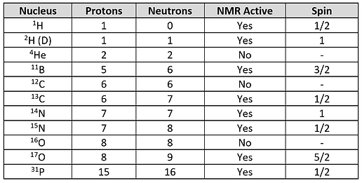
To understand the process of NMR, it is first useful to review the concept of spin in atomic nuclei. Subatomic particles (electrons, protons and neutrons) can be imagined as spinning on their axes. Most nuclei, the repository of protons and neutrons for each atom, have multiple spinning entities within. For many isotopes, the spins are paired against each other resulting in no overall spin of the nuclei. This occurs when both the number of neutrons and protons in the nucleus are even. However, nuclei with an odd number of protons and/or an odd number of neutrons will have an overall spin. The overall spin for those atoms that have an odd number of neutrons OR protons have a ½ integer spin (e.g. ½, 3/2, 5/2 etc…) while those with both an odd number of neutrons AND protons have an integer spin (e.g. 1, 2, 3 etc…). The latter case is less common. Nevertheless, all atoms possessing an overall spin are said to be ‘NMR Active’ with the most commonly utilized for analysis being 1H and 13C. The former gets much of the focus in the remainder of the discussion. Table 1 lists whether nuclei are NMR active or not as well as the overall spin for some common isotopes.
Table 1: Comparison of the number of protons, neutrons, NMR activity and overall spin for various atomic nuclei.
Nuclei actually have multiple spin states (i.e. spin configurations). The number of spin states for a nucleus can be determined by 2I+1 (from Quantum Mechanics) where I is the spin value. The spin value is 1/2 for both 1H and 13C. Thus, the number of spin states for both is 2, with the two individual spin states (m) defined as +½ and -1/2. These spin states have different energies when in the presence of a magnetic field.
The concept of different spin states having different energies can be better understood by first remembering that nuclei are charged particles (because of their positively charged protons) and moving electric charges generate magnetic fields. Thus, nuclei generate their own very small magnetic fields and can be thought of as behaving like a bar magnet. Figure 2 shows this analogy more clearly for a spin ½ nucleus.
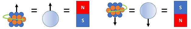
Figure 2: NMR Active atomic nuclei have an overall magnetic moment and can be visualized as a bar magnet whose north pole is oriented in the same direction as the nuclei magnetic moment.
Hypothetical nuclei containing a number of neutrons (blue spheres) and protons (orange spheres) are shown with the direction of spin represented by green arrows. The spin direction determines the orientation of the magnetic moment (the magnetic strength and orientation of a magnet) which is denoted by a black arrow. An atomic nucleus is often simplified with a single circle and an arrow pointing in the appropriate direction of the magnetic moment. The direction in which the magnetic moment points can be thought of as the north pole of a bar magnet. A group of magnets will be distributed randomly in the absence of a magnetic field. But when subjected to a magnetic field the nuclei will either align with or against it (see Figure 3).
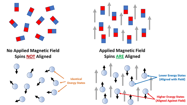
Figure 3: Atomic nuclei in solution represented by bar magnets (upper) and ball and arrows (lower). When no Magnetic Field is present, the spins are distributed randomly. But in the presence of a Magnetic Field the bar magnets align with (lower energy spin states) or against (higher energy spin states) the field.
This is similar to what happens within an NMR sample. In a solution, the spins of all nuclei comprising the sample are randomly distributed/aligned. The spin states under this condition all have the same energy and are said to be ‘degenerate’. However, when a magnetic field is applied the spin states obtain different energies with one being lower and the other being higher in energy than the original ambient spin states. The lower energy spin state (m= +1/2) has the nuclei oriented in the same direction as the magnetic field (defined as ‘parallel’) while the higher energy spin state (m= -1/2) has nuclei oriented against the magnetic field (defined as ‘anti-parallel’). The energy difference between the two spin states can be increased by increasing the applied magnetic field strength (see Figure 4). In NMR both sensitivity and spectral resolution improve as the energy difference increases. Thus, there are significant advantages to using stronger magnets for NMR analyses.
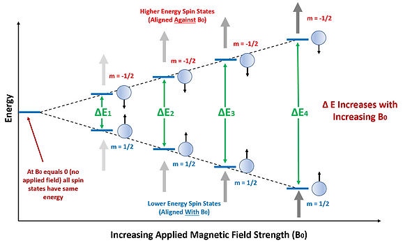
Figure 4: The energy difference between the two spin states increases with increasing strength of the applied magnetic field. The lower energy spin states are aligned with the field while the higher energy spin states are aligned against it. When no field is applied, all spin states have the same energy and no RF absorption can occur.
The Boltzmann Distribution can be used to calculate the ratio of nuclei in the high versus low energy states. The ratio is dependent on the magnetogyric ratio, a value specific to each nucleus, as well as variables including the temperature and magnetic field strength and the Boltzmann and Planck’s constants.

The population of the lower spin state relative to the upper spin state is only slightly higher under ambient conditions because the energy separation between the lower and upper energy levels is relatively small allowing thermal collisions to induce nuclei into the higher energy states. However, the energy difference can be increased by either LOWERING the temperature, which is not very practical, or INCREASING the magnetic field resulting in a GREATER excess of nuclei in the lower spin state (i.e. oriented with the Magnetic field). For example, for 1H in an external magnetic field of 9.39 Teslas (400MHz magnet) the ratio is 0.9999356. Here, 50.0016% of the nuclei are in the Low Energy state while 49.9984% are in the High Energy state. Increasing the magnetic field strength subsequently lowers the ratio (i.e. more atoms exist in the lower level spin state). Having a greater excess of nuclei in the lower spin state is advantageous in NMR as it ultimately allows for more signal (i.e. increased sensitivity) to be obtained since there are more nuclei available to absorb radio waves. Using an external field of 19.9 Teslas (850MHz magnet) decreases the ratio to 0.9998228, demonstrating how small the difference remains between the two states, even with a relatively high magnetic field applied. Thus, many multiple acquisitions are performed in a typical NMR experiment and the data averaged to improve the signal to noise ratio.
When a nucleus is irradiated with a frequency of electromagnetic radiation whose energy matches the energy difference between the two spin state levels, the spin states can flip with nuclei going from low energy level to high energy level resulting in energy absorption while the opposite direction results in a release of energy. It so happens that radio waves have frequencies (and thus energies) that are in the range necessary to induce these transitions between the two spin state energy levels. NMR measures which RF frequencies are absorbed by the sample and uses this information to determine its structural properties.
When the correct energy is applied, spin state transitions occur as energy is absorbed. But after a short period of time the number of nuclei in the lower and upper spin states are equal and the system is said to be saturated. No net absorption of energy occurs following this point. Thus, in modern day NMR instruments an RF pulse is applied to stimulate spin state transitions, reaching saturation, and then the system is allowed to ‘relax’ whereby which an excess of nuclei with lower energy states is again achieved before another pulse is applied. This process is repeated throughout an analysis and the data is combined and averaged for improved signal to noise ratios (see Figure 5).
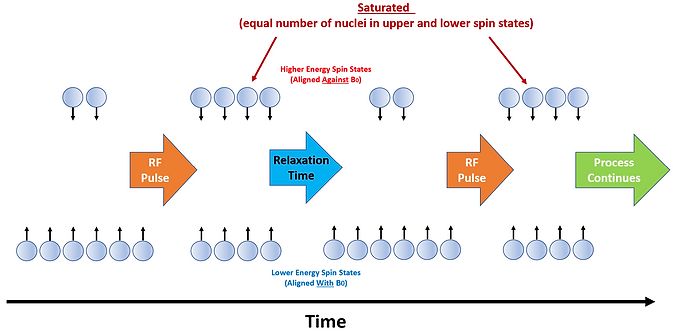
Figure 5: Schematic showing the RF Pulse process in NMR instruments. The RF Pulse results in a point of saturation whereby which there are equal numbers of nuclei in the Higher and Lower Energy States. A Relaxation step allows the Lower Energy State excess to reestablish so that the sequence can continue.
While the RF Absorption process can be visualized quantum mechanically in terms of the quantum energy of transition between possible spin states as described above, it can also be visualized by spinning tops that ‘precess’. The basis of this visualization is that spinning nuclei are unable to orient exactly with or against the applied magnetic field. They instead precess or wobble (like a gyroscope) about the axis of the applied field with a precession frequency (or Larmor Frequency) as shown in Figure 6.

Figure 6: Nuclei wobble (i.e. precess) about the axis of the applied field as does a gyroscope. The frequency of the wobble is known as the Precession Frequency.
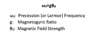
Radio waves have a frequency range consistent with the precession frequencies which is the number of times per sec that the nuclei precess in a complete circle. When RF radiation is applied to the spinning nuclei, absorption can occur when the applied radiation coincides exactly (i.e. resonates) with the nuclei precession frequency causing its spin to flip from an orientation with to one that is against the primary magnetic field. The precession frequency (ω0) is dependent on both the magnetic field strength (B0) and the nature of the nucleus.
1H has the largest magnetogyric ratio (also known as the gyromagnetic ratio) meaning that it exhibits the highest sensitivity in NMR making it extremely useful for the analysis of organic compounds which typically are laden with these atoms.
Nuclei can only absorb RF radiation that matches the precession frequency. This frequency is called the resonance frequency. NMR instruments are typically described in terms of their resonance frequency for a 1H nucleus. For instance, 2.3 and 25.8 Tesla magnets are defined as a 100 MHz and a 1.1 GHz spectrometer, respectively.
The ability of NMR to provide structural information arises from the fact that in an external magnetic field of a given strength, protons in different locations in a molecule have different resonance frequencies. This is because the nuclei are surrounded by orbiting electrons, which are charged particles, that generate their own small magnetic field that can add or subtract from the externally applied magnetic field. So, the electrons can partially ‘shield’ the nuclei with the amount being dependent on the exact local environment. Thus, for instance, a H bound to O will be shielded differently from that bound to N or C. These protons are in non-identical electronic environments and are said to be ‘Chemically Nonequivalent’. The presence of other more electronegative species pulls electrons from the C on which the H is attached effectively decreasing the electron density of their protons. These species ‘deshield’ the proton allowing it to ‘feel’ more of the external magnetic field. The general trend of electronegativity with atoms is found in Figure 7.

Figure 7: Comparison of electronegativity of selected elements important for NMR analysis.
General rules for chemical shifts are as follows:
1. The presence of electronegative species (e.g. O, Cl, N) as well as sp2 hybridized C (i.e. Carbon double bonds) result in deshielding and subsequently chemical shifts in NMR signals from species.
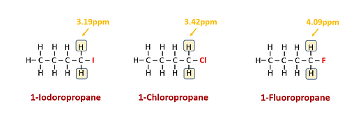
2. As the electronegativity of substituents increase, deshielding increases as well resulting in larger chemical shifts. (The concept of Chemical Shift is discussed in greater detail below.) For example, H on a C that also has F attached will have a larger shift than one that has Cl bound to it.
3. As the number of electronegative species on the C atom increases, deshielding increases accordingly. For example, H on a C that has 2 Cl atoms attached will have a larger shift than one that has only 1 F atom attached.

4. Deshielding decreases significantly with increasing distance from the atom of interest.
5. Protons involved in H bonding (i.e. those bound directly to O and N) do possess a chemical shift. However, the shift can vary significantly depending on a number of factors including the type of solvent and the concentration of the analyte.
Data
In NMR spectroscopy, a magnetic field is applied to a sample and the different amounts of energy required to induce resonance in the various nuclei comprising the sample are measured. NMR spectra is a measure of intensity (Y-axis) versus frequency absorbed (X-axis). The frequency is the precession or Larmor frequency (which is directly proportional to the Energy) of the applied RF electromagnetic radiation necessary to induce absorption (i.e. transition from lower to higher energy level) for the various NMR active nuclei present in the sample. Because this frequency is dependent on the magnetic field strength which can differ between instruments, the frequency is instead reported in NMR spectra as a ‘Chemical Shift’ (in ppm) which is the difference in the resonance frequency of a nuclei relative to that of a reference standard, typically TMS (trimethylsilane) in 1H NMR. TMS is commonly used as its protons are all chemically equivalent (thus only one signal appears) and are highly shielded such that very few organic compounds contain protons with chemical shifts negative to it.
Units of ppm are used in NMR spectra rather than Hz because the local changes in the applied magnetic field are several orders of magnitude lower than the actual field. Most protons in organic compounds have chemical shifts 0-13ppm from TMS. While this manner of referencing ensures that the units are equivalent across different field strengths (i.e. instruments), the actual frequency separation in Hertz scales with field strength (B0). Thus, machines with larger B0 result in spectra with peaks that are less likely to overlap. This increased spectral resolution has significant data interpretation advantages for analysis.
By comparing the chemical shifts of signals against chemical shift tables, possible structural environments can be determined (see Table 2).
Table 2: Chemical shifts for common proton bonding environments. Shifts denoted with an ‘a’ indicate that the value can vary with temperature, solvent and concentration.
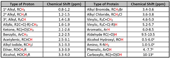
Species with higher chemical shifts (higher ppm values) are considered to be ‘downfield’ as the nuclei experience more deshielding and thus a higher exposure to the applied magnetic field. Those with lower chemical shifts (lower ppm values) are defined as ‘upfield’ and experience more shielding from the applied magnetic field (see Figure 8).
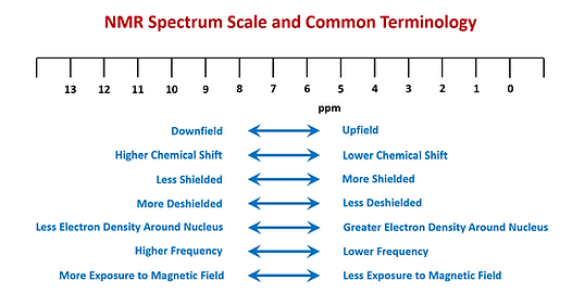
Figure 8. Common terminology used in NMR shown how they pertain to the NMR spectrum.
Since NMR is sensitive to the chemical environment of compounds, it is often easily able to differentiate between two or more with identical molecular formulae (i.e. isomers). As an example, Figure 9 shows 1H NMR spectra for 1-Chlorobutane (upper) and 2-Chloro-2-methylpropane (lower). Even though both have a molecular formula of C4H9Cl, their spectra differ considerably.
Various aspects of an NMR spectrum reveal important information about the sample. They are as follows:
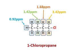
Number of Signals: Counting the number of signals present determine how many distinct proton environments exist in the sample. Thus, the number of different sets of protons can be determined. For example, there are 4 distinct chemical environments for 1H in 1-Chlorobutane but only 1 in 2-chloro-2-methylpropane. Thus, the former has 4 sets of signals while the latter only 1. The H atoms in each different chemical environment in the figures are highlighted with a different color and their subsequent set of peaks are highlighted accordingly. For example, the 2 H atoms adjacent to Cl in 1-Chloropropane and highlighted yellow are chemically equivalent and form the set of peaks at 3.42ppm in the spectrum. H atoms found further down the C chain have different chemical environments and correspondingly different chemical shifts.
Position of Signals Along X-Axis: Determines the magnetic environment of each proton set. This identifies the type of proton present based on chemical shift charts (discussed earlier). For 1-Chloropropane the influence of the electronegative Cl atom on the H atoms decreases steadily down the C chain, resulting in less shielding and smaller chemical shifts. It is interesting to note that the chemical shift for the H atoms of 2-Chloro-2-methylpropane is almost identical to that for the H atoms highlighted in orange for 1-Chloropropane. Both sets of H atoms are found on C atoms adjacent to the C atom bound to Cl.
Splitting Pattern (Multiplicity), Coupling, Signal Splitting: In 1H NMR, when 1H nuclei have adjacent atoms with nonequivalent H atoms, those H atoms can split the energy levels of the 1H resulting in multiple peaks rather than a single signal. This splitting (also called coupling) follows well defined rules, namely signal = n+1 where n is the number of nonequivalent vicinal hydrogens. Thus, the splitting pattern of each signal determines the number of H atoms present on C atoms adjacent to those producing the signal, a further useful tool in determining the structure of compounds being studied.
The spectrum of 1-Chloropropane shows this splitting more clearly. Both the yellow and blue highlighted H atoms have two adjacent non-equivalent H atoms. Thus, the resulting signal is a set of 3 peaks at 3.42ppm and 0.92ppm, respectively. The orange highlighted H atoms, on the other hand, have four adjacent non-equivalent H atoms and the resulting signal has 5 peaks. The green highlighted signal has 6 peaks because there are 5 non-equivalent H atoms on adjacent atoms. For 2-Chloro-2-methylpropane, a single peak is observed (i.e. no splitting is observed) since all of the H atoms are chemically equivalent and there are no non-chemically equivalent H atoms on adjacent atoms.
Area Under the Signals: In 1H NMR, the relative peak areas indicate the relative number of protons producing each signal. This can be useful in helping elucidate the structure of a compound. For example, the blue highlighted signal set for 1-Chloropropane is more intense than the yellow set due to the former resulting from 3 H atoms and the latter only 2. The green and orange highlighted signal set also only contain 2 H atoms each but are more difficult to compare visually to the others as they are composed of multiple peaks. Thus, peak area calculations are needed for their comparison.
Peak areas can also be used to determine relative amounts of compounds in a mixture where all compounds present contain 1H nuclei in distinct chemical environments from one another.

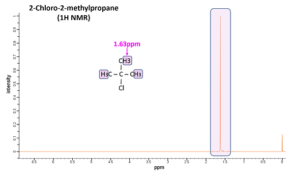
Figure 9: 1H NMR spectra of 1-Chloropropane (upper) and 2-Chloro-2-methylpropane (lower). Both are expanded view as the regions between 4.5-13.0ppm are featureless. H atoms within the same chemical environment are shaded with the same color as are the resulting peaks.
Instrumentation
There are two general types of NMR instruments, Continuous Wave and Pulsed (or Fourier Transform) NMR. Continuous Wave instruments were the original NMR spectrometers and worked by applying a weak RF input at constant frequency while applying a variable magnetic field or vice-versa. These instruments are rarely used today. Instead, Pulsed NMRs dominate the high-end area of the market. One such instrument manufactured by Bruker is shown in Figure 10 helping to put the size of an NMR into perspective. Note that table top instruments are also manufactured but these have much lower Magnetic Fields and lack many of the capabilities of the high-end tools. They are, however, considerably cheaper making them within the budget of a larger number of labs.
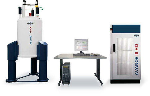
Figure 10: Image of 600MHz NMR tool manufactured by Bruker.
In the modern-day pulsed NMR analysis, the sample is placed in the center of a strong, homogeneous magnetic field causing the NMR active nuclei to align with or against the magnetic field. Increasing magnet strengths result in both increasing sensitivities and spectral resolution, thus the impetus for using as strong of a magnetic as possible. A superconducting magnet is used to create the strong applied magnetic field, B0. Magnets as large as 25.8T are now found in the most advanced modern NMR instruments, but most commercial instruments range from 9.39-19.9 Teslas. (Table top instruments have considerably smaller magnetic strengths.) The magnet typically consists of solenoid coils made from metal alloys such as NbTi or (NbTaTi)3Sn formed into filaments and encased in Cu to protect the brittle alloys.
In order to have superconducting properties the magnet must be kept at extremely cold temperatures which is accomplished with a series of dewars and vacuum chambers (see Figure 11). The inner dewar, which contains the superconducting magnet, is filled with liquid He (4.2K, -269C). It typically must be filled approximately every 6 months. The inner dewar is encased in a vacuum space filled with radiant insulation (typically Al or reflective mylar) followed by a second dewar filled with liquid N2 (77K, -196C) to help minimize evaporation of the very expensive liquid He. The liquid N2 dewar is typically refilled every 1-2 weeks although Bruker offers a ‘Nitrogen Re-liquefaction Accessory’ that alleviates boil off of the liquid N2 thereby eliminating the need for N2 refills. Finally, the entire system is encased in an outer vacuum compartment to further minimize liquid N2 and He evaporation.
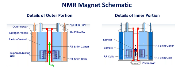
Figure 11: Schematic of the Outer and Inner Portion of an NMR Magnet. (From Bruker)
Samples are most often dissolved in a solvent which either contain no H or is deuterated to avoid an intense, potentially interfering 1H signal from the solvent. (Note, that solid samples can be analyzed for certain applications.) These liquid samples are placed inside a tube (typically 1-10mm in diameter and 2-20.3cm in length) made of an inert material (e.g. glass, quartz, PTFE) which sits inside a removeable probe surrounded by shimming coils all located within a compartment in the center of the superconducting magnet. The shimming coils are used to create additional magnetic fields to counter any inhomogeneities present in the primary magnetic field, B0, which is necessary to obtain ultimate spectral resolution. The probe is capable of spinning the sample tube to further minimize the effects of magnetic field inhomogeneities.
The probe contains a set of coils whereby which very short RF pulses (microsecond range) are delivered to the sample via a Frequency Generator/Transmitter. This RF pulse generates an additional, temporary magnetic field, B1, orthogonal to the primary magnetic field. This temporary B1 applies a torque to the nuclear spins of the sample nuclei, twisting them out of alignment with B0 and causing them to undergo precession where they acquire rotational motion (like a gyroscope) around B0.
The induced precession frequency is equal to the resonance frequency or energy difference between the upper and lower spin state energy levels. Each RF pulse has a broad spectrum of radio frequencies capable of matching the resonance frequencies (i.e. can induce spin state transitions) of all the NMR active nuclei of interest. This is important as the resonance frequency is not only dependent on the magnetic field strength and the type of atom, but also the local environment and position of the nuclei within the molecule. Thus, the precession frequency for each distinct type of nuclei contains valuable information on the structure of a molecule making it important that all are measured. The precessing nuclei induce an alternating voltage in a coil within the probe surrounding the sample and holder. The signal is an overlay of multiple oscillating electric signals from all the NMR active nuclei within the sample, each with a frequency corresponding to the precession frequency (i.e. resonance frequency) from the specific nuclei in which it was generated.
Once the RF pulse ends, the Free Induction Decay (FID) is measured which is the signal produced by the sample as the nuclei relax back to their original state of alignment with B0. This decay, characterized by a progressive decrease in the signal voltage, typically only takes a few seconds and the measurement is signal intensity versus time. The resulting signal is fed into a preamplier (since the signal is inherently weak) and then a Demodulator, to remove the RF pulse signal, followed by a Digitizer. A Fourier Transform (a mathematical manipulation) of the signal is performed to convert it from a time domain into a frequency domain producing the conventional NMR spectrum where the characteristic frequencies of the precessing nuclei appear as distinct peaks (i.e. resonance lines). The shift of these signals from a reference position, their splitting patterns and intensity are used to deduce structural information on the molecules present. Figure 12 shows this process for both one NMR active signal and for the more realistic scenario of multiple NMR active signals.
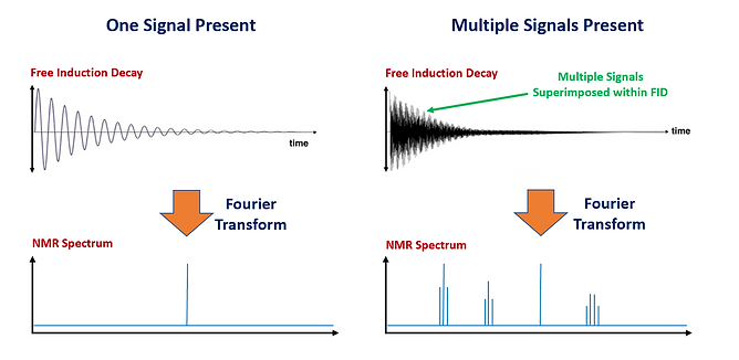
Figure 12: The Free Induction Decay and Subsequent Fourier Transform to produce the NMR spectrum is shown on the left side for one NMR active signal and on the right side for multiple NMR active signals.
Other NMR Techniques
C13 NMR
While much of the discussion above has focused on 1H NMR, 13C NMR is also commonly employed to provide additional valuable insight into the nature of organic samples. This can be particularly useful for larger molecules. However, there are additional challenges with 13C relative to 1H NMR. First, the 13C isotope is only ~1% of all C atoms. Second, the magnetic moment of 13C is much weaker than that of 1H. These factors result in a much weaker signal in 13C and consequently more S/N averaging is necessary.
As in its proton counter-part, chemical shifts are used to identify the type of C present in 13C NMR. However, 13C nuclei resonate at a different frequency (~75MHz versus ~300MHz in a 300MHz instrument) than that of 1H resulting in it appearing in a different energy window. TMS is also used as the internal standard but for 13C NMR the shift from the C nuclei is measured. The range of chemical shifts in 13C NMR is considerably larger (~200ppm) compared to that of 1H NMR (~12ppm) resulting in less signal interferences. Differences in the magnetic environment are again the source of the chemical shift from the TMS standard with electronegative atoms, diamagnetic anisotropy and sp2 hybridization causing signals to shift downfield. Figure 13 shows 13C NMR spectra for 1-Chloropropane and 2-Chloro-2-methylpropane. As was observed with the H atoms in 1H NMR, the C atoms further from the electronegative Cl atom of 1-Chloropropane have smaller chemical shifts. Four signals are observed as there are four different C environments. While there was only 1 signal in the 1H NMR spectrum for 2-Chloro-2-methylpropane, there are 2 signals in the 13C NMR as there are 2 distinct C chemical environments.
Spin-Spin coupling is not observed in 13C NMR since their relatively low abundance results in it being highly unlikely that the 13C nuclei are adjacent to one another. (Notice only one peak is observed for each signal in the 13C NMR spectra of Figure 13.) However, heteronuclear coupling between 13C and the Hs bound to them does occur although broadband decoupling is typically used to remove C-H coupling so as to simplify the spectra. Nevertheless, Distortionless Enhancement by Polarization Transfer (DEPT) is often used to determine how many H atoms are bound to each C nuclei responsible for signals in the spectra.
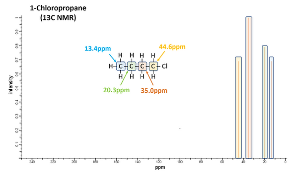
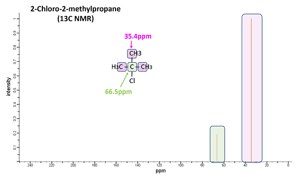
Figure 13: 13C NMR spectra of 1-Chloropropane (upper) and 2-Chloro-2-methylpropane (lower).
Multi-Dimensional NMR
In addition to conventional NMR, multi-dimensional NMR (i.e. 2D, 3D and 4D NMR) is commonly performed for compounds that give complicated NMR spectra containing partial and/or completely overlapping signals in conventional NMR (e.g. heteropolymers, biological macromolecules). It is also often used for the analysis of mixtures. In conventional (1D) NMR, the output is a simple 2 axis spectrum plotting Intensity versus Frequency. As the name implies, Multi-Dimensional NMR adds additional frequency axes. In 2D NMR, a plot of frequencies on both the x and y axes is obtained. This plot allows one to determine which signals are actually ‘coupled’ to one another, in other words which ones affect the magnetic environment of another. Homonuclear methods involve coupling between the same type of nuclei (e.g. 1H and 1H) while Heteronuclear methods involve coupling between different types of nuclei (e.g. 1H and 13C).
Solid State NMR
As mentioned earlier, samples are typically run as liquids as this form provides the best quality data. However, there may be some samples that are not amenable to liquid form (e.g. can’t be dissolved) or must be analyzed nondestructively (e.g. expensive biological nucleic acids or proteins). For these the samples can be analyzed as a solid and such analysis is referred to as Solid State NMR. SSNMR tends to have poorer sensitivity and resolution than solution NMR. Historically, SSNMR experiments have tended to be more specialized and complicated over the general-purpose liquid NMR. However, improvements in instrument design such as rapid sample spinning to improve spectral resolution have now resulted in a wider array of applications.
Comparison
When characterizing a newly synthesized organic compound chemists often rely on a number of analytical techniques including NMR, Mass Spectrometry and Infrared Spectroscopy. These techniques provide very complementary and unique information and when taken together can paint a complete picture of the material.
Mass Spectrometry is used to provide the molecular formula of the compound. Fragmentation patterns are also useful in providing some structural information. Infrared Spectroscopy is used to provide the functional groups/chemical bonding that is present. 1H NMR provides the chemical environment of the Hs present in the compound, the number of Hs giving rise to the resonance and the number of non-equivalent Hs on adjacent carbons. 13C NMR provides the number of individual C species present.